Sensory - Motor Practical Neurosystems
by Dr. Tonny Mulder and Dr. Julia Dawitz

SENSORY - MOTOR PRACTICAL
In this practical you are going to examine the link between what enters the brain, the processing of this information and the behavioral output.
You will perform a behavioral auditory Go-NoGo task and record prefrontal and parietal cortices (EEG) in order to get a grip on the processing of this auditory information. Furthermore, to investigate the timing and accuracy of the behavioral output the activity of the motor and frontal cortex (EEG) and hand muscles (EMG) are recorded. Lastly, eyeblinks (EMG) and heartbeat (ECG) will be measured.
Before you can start with the actual experiment you will first examine a number of important principles that are essential for the interpretation of the results.
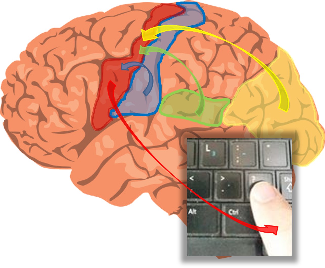
From sensory systems via the motorcortex to the keypress.
In a behavioral task where you press a key in response to a cue, sensory systems detect the cue and the corresponding muscle activity is regulated by the motorcortex (See picture to the left). The motor cortex has a topographical layout regarding the control of various muscles. Its axons run, amongst others, via the pyramidal track down to the ventral horn, synapsing on the large motor neurons of the spinal cord. These motor neurons innervate the muscles of the hand and fingers. The muscles move fingers across the key pad, producing this introduction to the experiment.
All this information is transmitted via neuronal actions which can be visualized by EEG, recorded with the EEG equipment. In addition this system can record muscle activity, the ElectroMyoGram (EMG).
In this practical activation of sensory systems will be recorded and the coupling between motor cortex and muscle activity examined. In addition heart beat (ElectroCardioGrams (ECG)) and eyeblinks (ElectroOculoGrams (EOG)) will be measured, both related to attention and stress.
Succes and lots of fun
There are four modules in total. Each module starts with the general information, after which you can start. Module I will be dealt with in a self study assignment, whereas module II and III are 'On-Campus'. The fourth analyse module gives you a preview of data analysis.
Don't skip information, so read read read before diving into a module. Also when stepping through the module it is important to read!
Click on one of the button below to start a module
Module I
The principles of EEG recording
Module II
Your first recording
Module III
Sensori-motor experiment
Module IV
EMG analyse
Module I
From the analog brain to the digital PC
Tijdens dit eerste experiment maken jullie kennis met de omzetting van een analoog elektrisch signaal naar digitale data dat door de computer kan worden opgeslagen. Er vinden een aantal essentiële stappen plaats die invloed kunnen hebben op hoe je data er uiteindelijk uitziet en die je daarom moet begrijpen om je data te kunnen interpreteren. De hier beschreven stappen gelden overigens niet alleen voor EEG en EMG maar worden ook toegepast bij het meten van extracellulaire afleidingen, zoals jullie die in het wormenpracticum hebben gemeten.
Om de signalen te kunnen meten zijn er 3 basisstappen nodig: Versterken, Filteren en de Digitalisering van het signaal.
In dit eerste experiment gaan jullie de mogelijke invloeden van deze stappen aan de hand van vragen zelf onderzoeken. Voor elk experiment is er een CANVAS antwoord document waar de antwoorden op kunnen worden ingevuld. Lees eerst de tekst en volg de instructies op de website en beantwoord daarna de daarop volgende vragen binnen CANVAS.
Gebruik CANVAS om de vragen bij MODULE I te zien en maak de quiz!
Begin nu met Stap 1
Stap 1: Versterken
Stap 2: Filteren
Stap 3: Digitaliseren
Stap 4: Uitmiddelen
Versterken van het signaal
Het signaal wordt versterkt zodat het groot genoeg is om door de apparatuur gemeten te worden. Dit gebeurt hier in de g.MOBIlab versterker. Elke versterker heeft specificaties (Afbeelding 2). Deze bepalen de marges waarbinnen je met deze versterker kan meten.
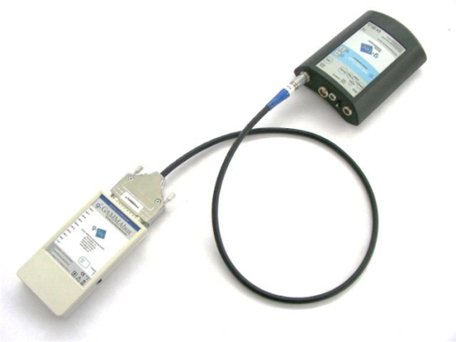
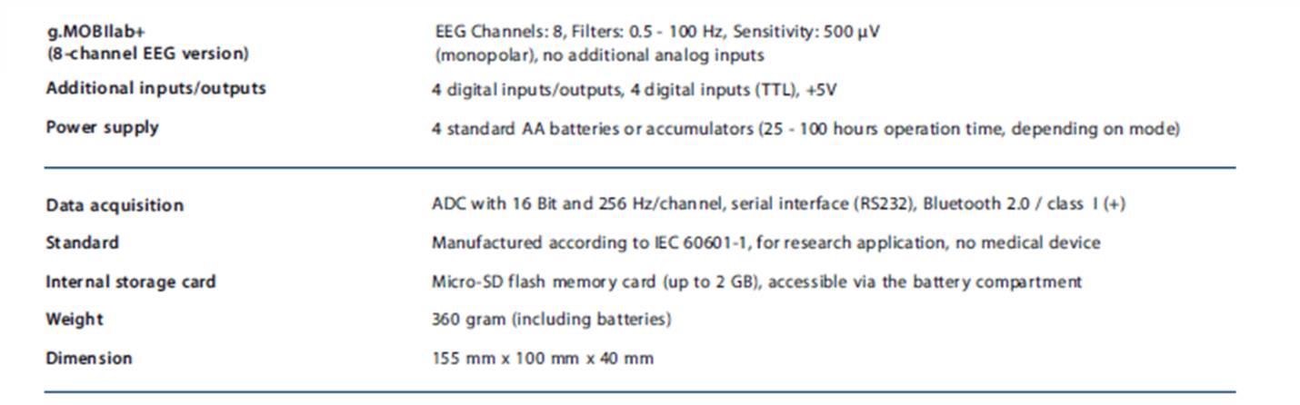
Figuur 2: De EEG versterker (links) en de specificaties van het systeem (rechts).
Maak Vraag I.1 tot en met I.4 van de QUIZ: Motoriekpracticum Experiment I: van het analoge brein naar de digitale PC
Filteren van het signaal
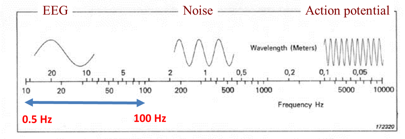
Als het ruwe signaal binnenkomt, is het vaak niet 'schoon'. Dwz, het bestaat uit een deel van interesse en een deel uit ruis (noise) en artifacten. Ruis is in dit geval gedefinieerd als alle frequenties waar we niet in geinteresseerd zijn. Artifacten zijn externe verstoringen, zoals de 50Hz vanuit het lichtnet.
Wat je als signaal ziet en wat als noise dat verschilt per experiment. Voor een EEG/EMG meting worden alle frequenties hoger dan 100 Hz als noise gezien maar tijdens het wormenpracticum zijn alle frequenties lager dan 1000 Hz noise. Daar lag de interesse op de actiepotentialen.
Om ruis te verwijderen filter je deze uit je signaal. Dat gebeurt meestal in twee stappen.
Stap 1 zit vaak in de versterker ingebouwd en is onderdeel van de versterker specificaties (zie figuur 2). De gebruiker heeft daar geen invloed op, behalve door de juiste versterker te kopen voor het experiment.
Stap 2 staat onder de controle van de gebruiker, die on-line (tijdens de meting) of off-line (na de meting) verder het signaal kan filteren en daarmee opschonen.
Het signaal wordt in de MobiLab versterker gefilterd van 0.5 tot 100 Hz, dmv een bandpass filter. Alle frequenties tussen de 0.5 Hz en 100 Hz wordt doorgelaten en de rest wordt geblokkeerd (Zie afbeelding 3a).
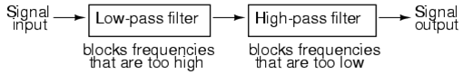
Figuur 3a: Het toepassen van een bandpass filter. Eerst wordt het signaal door een Low-pass filter gestuurd en daarna door een High-pass filter. .
Op deze manier kan je het EEG signaal isoleren van storende, in dit geval Noise en Actiepotentialen. (Zie afbeelding 3b).
Figuur 3b: De filter settings van de MobiLab versterker en het effect op het ruwe signaal.
Maak Vraag 1.5 tot en met 1.7 van de QUIZ: Motoriekpracticum Experiment I: van het analoge brein naar de digitale PC
DIGITALISEREN VAN HET SIGNAAL
Introductie
De signalen die door de hersenen en de spieren worden geproduceerd zijn analoge, continue, signalen. Met computers is het niet mogelijk om een continu signaal op te slaan; een computer werkt digitaal. Het analoge signaal wordt gesampled met een bepaalde resolutie. Alleen deze gesampelde punten worden opgeslagen en de tussenliggende data gaat verloren. Zowel in de tijd (sample frequency) als in de amplitude (bit levels) wordt gesampled.
Jullie kennen dit van foto’s, uit het spatiële domein. Als je een digitale foto maar ver genoeg inzoomt zie je op een gegeven moment de vierkante pixels waaruit de foto is opgebouwd. Elke pixel geeft het gemiddelde weer van de informatie die binnen deze pixel is binnengekomen. Dingen die op dezelfde pixel zijn binnengekomen zijn niet van elkaar te onderscheiden, de spatiële resolutie van de foto is dan te laag om deze verschillen te zien (Afbeelding 4).


Afbeelding 4: Een digitale foto is opgebouwd uit pixels. Links, foto van gebouw H0.08 van het Science Park (UvA). Rechts, ingezoomd op de fiets die rechts naast het gebouw staat. De pixels zijn duidelijk zichtbaar. De spatiële resolutie van de foto laat het zien van details (zoals aan- of afwezigheid van een bel) niet toe.
Als we de analoge signalen van de hersenen en de spieren willen meten, maken we gebruik van digitale apparatuur, en krijgen we te maken met de omzetting van continue (analoge) naar digitale signalen. Zowel de tijd (sampling frequency) als de amplitude (aantal bit levels) wordt gesampled. De data tussen de samplepunten in wordt niet omgezet naar het digitale domein en gaat verloren. In de computer worden de individuele samples met elkaar verbonden door rechte lijnen. Dit is dus niet identiek aan de werkelijke waardes van het continue signaal. De betrouwbaarheid van het verkregen digitale signaal hangt dus af van de sampling frequentie en het aantal bit levels. In de volgende tutorial gaan we spelen met de 'sampling frequency' en laten het aantal bit levels even met rust.
OPDRACHT
Hiervoor heb je MATLAB nodig, dat je reeds gebruikt hebt tijdens jaar 1 Neuroanatomie en Neurofysiologie
Nu gaan we bestuderen welke invloed de meetfrequentie (sampling frequency) heeft op het digitale signaal dat uiteindelijk op ons scherm verschijnt. Het signaal dat we later voor analyse gaan gebruiken.
Als het goed is heb je reeds het sampling programma gedownload van CANVAS en staat het nu al op je laptop. Zo niet doe dat dan alsnog. Ga dan door met het openen van MATLAB
Download het programma sampling.m en sampling.fig van CANVAS (het is een zip file). Plaats de zip in een folder op je DESKTOP of op een logische plaats op je laptop.
UNZIP de file
Open MATLAB
Stuur MATLAB naar de folder waar je het sampling programma hebt gedownload en geunzipped. Je Current Folder ziet er dan ongeveer zoals op afbeelding 5 uit.
Type het woord: sampling in je ‘Command window’ en druk op enter. Het programma wordt geladen en opent!
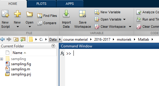
Afbeelding 5: Matlab interface. Screenshot van de ‘Current Folder’ van Matlab. In de adresbalk moet de folder staan waar jij sampling.m en sampling.fig hebt neergezet.
Voor het gemak gaan we ervan uit dat ons (analoge) input signaal een sinus met een bepaalde frequentie is, echter voor complexe signalen zoals hersengolven en spierpotentialen geldt de samenhang die we nu uitwerken ook.
Voer nu in: een analog frequency van 20 Hz en een sampling frequency van 400 Hz, Gebruik de 'show lines between samples' functie en sample de data.
Maak Vraag 1.8 tot en met 1.10 van de QUIZ: Motoriekpracticum Experiment I: van het analoge brein naar de digitale PC
N.B.: In de 'sampled data' plot in de simulatie wordt de lijn tussen de gemeten punten door het programma zelf ingevuld. Hetzelfde wordt gedaan tijdens het digitaliseren van EEG data. Deze verbindingslijnen worden geplaatst om ons het idee van een continue signaal te geven. We kunnen er worst van maken.
Dit is dus geen gemeten data. Zet de 'show lines between samples' functie maar eens uit. 'Its a sinus but not as we perceive it'
Als we een signaal bekijken willen we vaak twee dingen weten: Wat is de frequentie van het signaal en wat is de amplitude?
Ga nu het analoge 20 Hz, 1 mV input signaal met steeds lagere frequenties meten. Gebruik de volgende meetfrequenties (sampling frequencies): 400 Hz, 200 Hz, 100 Hz, 40 Hz, 20 Hz, 10 Hz, 5 Hz.
Gebruik voor deze opdracht: 'Keep Sample plots' om meerdere metingen over elkaar heen te plotten. Zet je deze optie weer uit dan verschijnt er de volgende keer dat je data ‘meet’ weer maar één plot.
'Clear plots' verwijderd alle geplotte data.
Maak Vraag 1.12 tot en met 1.17 van de QUIZ: Motoriekpracticum Experiment I: van het analoge brein naar de digitale PC
We hebben nu gezien dat een (te) lage sampling frequency invloed kan hebben op ons meetresultaat. De EEG apparatuur die we gebruiken om de spieractiviteit (en later ook de hersensignalen) te meten heeft een sample frequentie van 256 Hz (of zoals het in de software staat aangegeven 256 ‘samples per second’).
VOOR DE VOLLEDIGHEID: onze Mobilab versterker heeft in het amplitude domein een resolutie van 216 bit levels. Dat betekent dat de maximale amplitude range die we kunnen meten met onze versterker verdeeld wordt in 65535 samples. Gezien de input range van onze versterker 1 mV bedraagt is de amplitude resolutie 0.015 microV.
UITMIDDELEN VAN HET SIGNAAL
Introductie
In voorgaande opdrachten hebben we binnen het EEG signaal gekeken naar de frequenties die zich daar voordoen en daarvan de amplitudes. Er is echter nog een compleet ander veld van onderzoek dat zich bezig houdt met EEG signalen die ontstaan naar aanleiding van events (gebeurtenissen). Deze tak van sport meet 'event related potentials' of te wel ERPs. ERPs hebben een zeer kleine amplitude, tenopzichte van de 'sterke' hersengolven gerelateerd aan bv alpha, beta frequenties.
Om deze zichtbaar te maken is het noodzakelijk om de events vaak aan te bieden waardoor we een gemiddelde reactie van het brein op een bepaald event kunnen visualiseren. De volgende Zelfstudieopdracht, op CANVAS is er om dit proces duidelijk te maken.
Ga nu naar CANVAS en vervolg daar met de zelfstudie: Het verkrijgen van een mooi ERP
Module II
Now that we have an understanding of the theory underlying an EEG recording, it is time to record your first real EEG data. The purpuse of this experiment is to get acquintaint with:
- The EEG setup
- The signals that can be measured.
- The quality of the signals.
First of all we are going to record muscle potentials (EMG) of the lower arm, the electrocardiogram ( ECG) and the EEG of the prefrontale cortex.
Gebruik CANVAS om de vragen bij Module II te zien en lever per groep de antwoorden op de quiz in!
Maak Vraag II.1 en II.2 de QUIZ: Motoriekpracticum module II: De eerste EEG/EMG/ECG meting
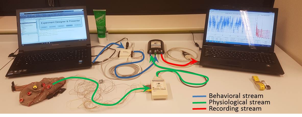
All materials lie befor you on the lab table and the EEG setup is already connected.
Scan the picture below to identify essential components
For the experiment of Module II we need:
- Recording equioment (On the right)
- The recording laptop
- Four red EEG electrodes (Voor dit experiment zitten ze niet in de EEG Cap)
- One yellow ground electrode
- The blue reference electrode
- Electrode stickers, tape, EEG gel and an syringe
Identifying setup components
Check if everything is there...
AND.... Check the connections
AND.... Got it all?
STARTING UP the EQUIPMENT
For now, only the EEG_Recorder laptop will be used
The EEG Recorder software is already downloaded and available on your EEG_Recorder laptop.
The latest version = ......... SEE your Recorder laptop
Start EEG_Recorder in MATLAB (32bits)
- Check if WIFI is available, on the recording Laptop. This is necessary for MATLAB license verification.
- Start MATLAB (32bits)
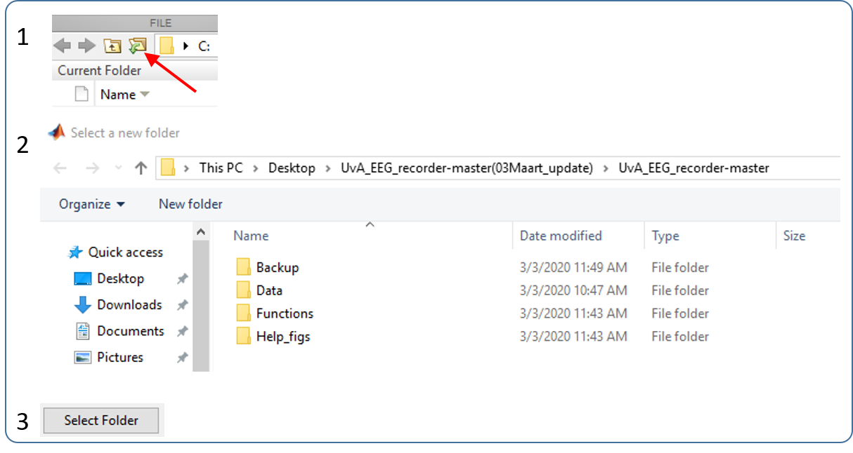
- Make the content of the EEG_recorder folder, the current folder. See example on the right.
Switch your Mobilab amplifier on
- This to be able to test your connections later
- You can find your Mobilab amplifier in the picture above
START THE PROGRAM
- - by typing ‘eeg_recorder’ in the command window
- - by dragging eeg_recorder.m to the command window
- - Via the edit Mode. DANGER: ONLY USE THIS OPTION IF YOU REALLY WANT TO EDIT. Double clicking eeg_recorder.m and then clicking on the green ‘Run’‐button. This opens the eeg_recorder.m file in the editor.
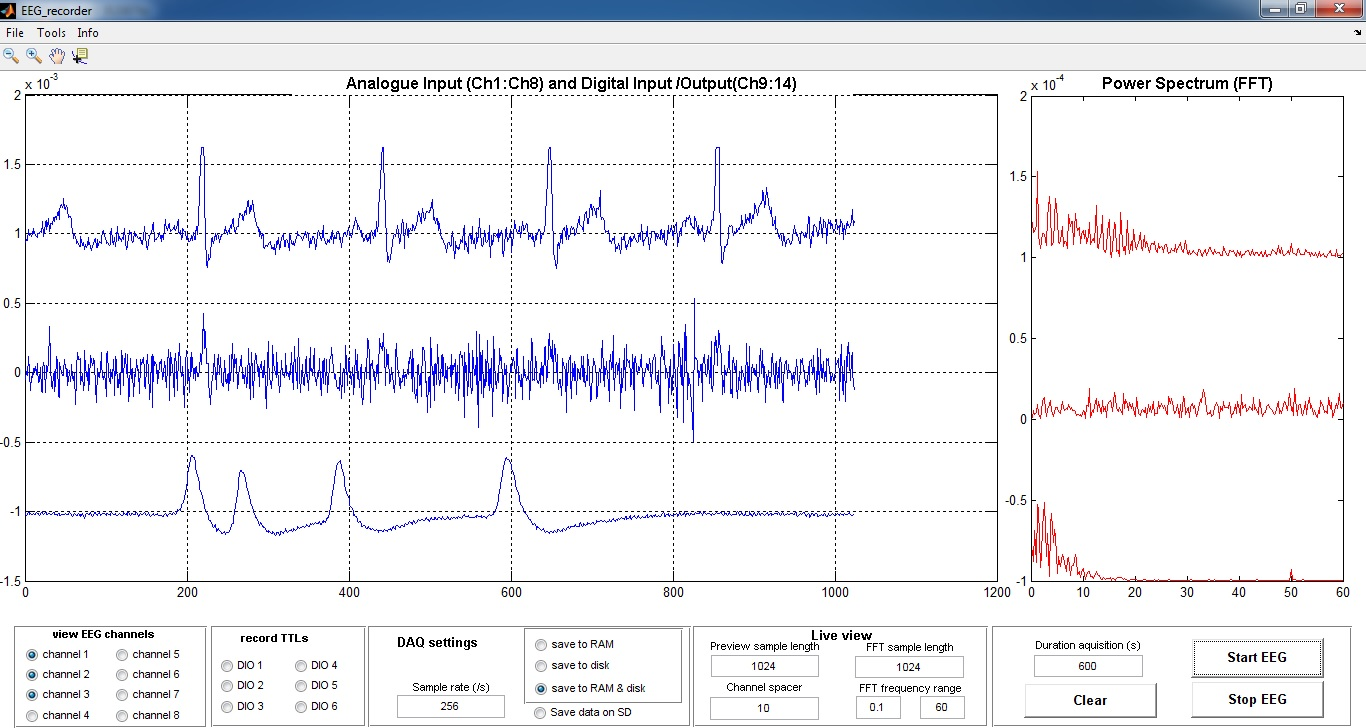
After loading the program, this is how the recording window should look, more or less!
In the latest version, however, colored buttons have been added and analyse tools have been updated.
EEG_recorder contains the following main functions:
- Record EEG
- Generate a live view of EEG in time domain and frequency domain
- Saves/Loads EEG to/from RAM and hard disk
- Analyze EEG data using several toolboxes
CONNECTING the ELECTRODES
Read through the connecting procedure below, BEFORE actually starting it
- Select a subject to record from
- Find the GAMMABox as part of the setup. Connected are:
- 4 red recording electrodes
- 1 yellow ground electrode.
- 1 blue reference electrode.
- Sticker the 4 recording electrodes
- Place two recording electrodes on the right arm:
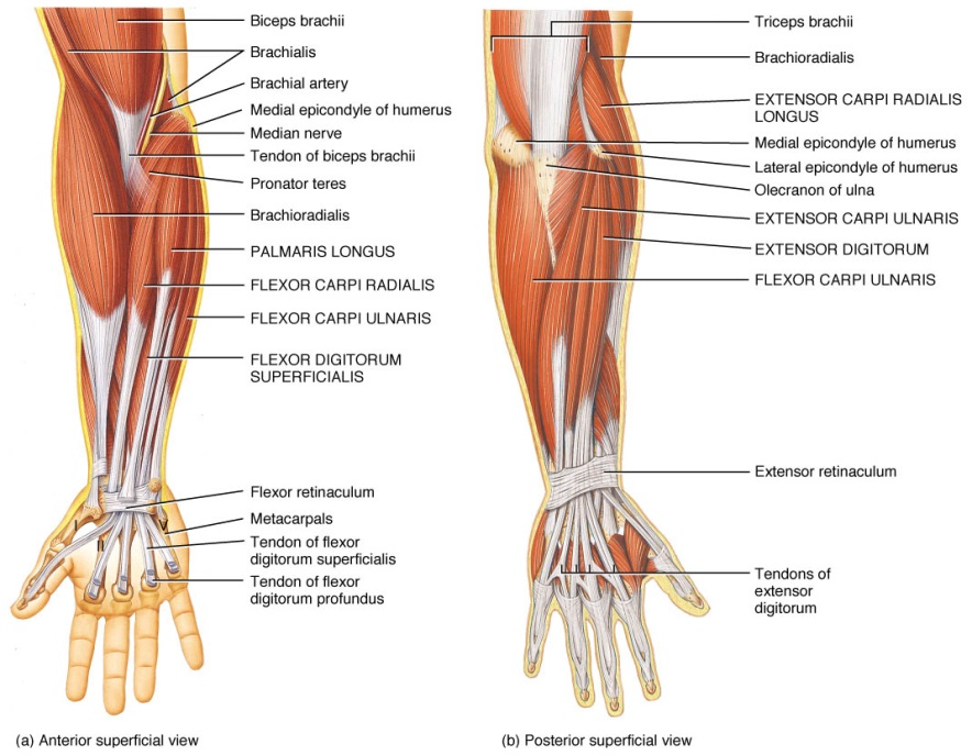
- Stick electrode 1 on the Extensor Digitorum (image 7) Find it by making a fist and move your wrist upwards.
- Stick electrode 2 on the Palmaris Longus (image 7). Find it by making a fist and move your wrist downwards.
- Connect electrode 3 on the left wrist. Turn your palm up, so your thumb points to the left. Stick the electrode about 3 cm beneath the wrist joint, left of the central tendons, the location where you can feel yoiur heart beat.
- Now connect electrode 4at a central location on the fore head, with the wire pointing horizontally to the right.
- Stick the yellow ground elctrodenext to the central PFc electrode on the forehead, with the wire pointing horizontally to the right.
- Tape al the wires to tye skin, releaving the tension on the electrode.
- Stick the wires behind the right ear of the test subject.
- Fill tye syringe with the contact gel and fill the electrodes with the gel (see image on the left).
- Place a small drop of gel on the blue reference electrode and clip it on the right earlope (see image on the right).
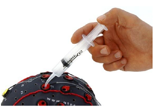
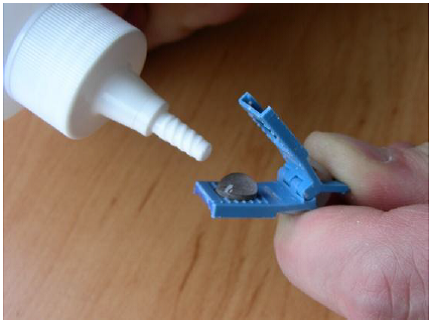
Image: Gelling electrodes.
SETTING the RECORDING-COMPUTER
We will use predefined setting. An extensive explanation can be found here > > > > > > > > > > > > >
SETTING the RECORDING-COMPUTER Module II :
When electrodes are connected, the signal can be tested. When looking at the recording program, all EEG and all marker channels are switched on by default. "Just to be save".
Swich of the ones that we dont need now. (see image 8).
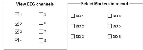
Image 8: Selecting EEG and marker channels in EEG_Recorder.
- Activate channels 1 through 4, turn off channels 5 through 8 . See Image! 4 red electrodes are connected so 4 channels need to be recorded.
- NOTE: the yellow ground and the blue reference electrodes just serve as ground and reference for all recording elctrodes.
- Turn all markers (DIOs) off, See image 8. For now we dont use them.
LIVE VIEW PANEL
Use the ‘Live view’ panel to adjust the screen settings. These settings do not change anything on the recorded and logged data.
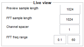
Image 9: The interactive ‘Live view’ panel of the EEG_Recorder.
- ‘Preview sample length’ = 1024 samples. So, 1024 data points are shown on the screen. With a sampling rate of 256 samples/s, this allows 4 seconds of data to be pushed to the screen.
- ‘Channel spacer’ default = 1. The smaller the channel spacer, the larger the amplitude of te signals. Keep the Channel Spacer to 1.
- Keep the ‘FFT sample length’ equal to the ‘Preview sample length’. The FFT is than calculated over the signal part that is shown on the screen.
- The ‘FFT frequency range’ is set from 0.1 to 60 Hz
A short explanation on Fast Fourier Transform
EEG and also EMG is recorded in the time domain . The raw signal (Voltages) is presented on a time line (the x-axis). This is the left 'raw EEG window' of the EEG-Recorder program.
A fast fourier transformation (FFT) recalculates the EEG signal from the time domain to the frequency domain. This means that per time block (epoch) the strength (Power) of every frequency is calculated and presented. Such as the delta, theta, alpha, beta and gamma frequencies that you might have heard of. See the 'FFT window' of the EEG-Recorder program above.
By setting 'Preview sample length' as well as the 'FFT sample length' at 1024 samples (4 seconds), the FFT is calculated over the piece of data that is presented in the time domain window.
Please realize that the EEG signal is complex whereby Alpha, Beta and Gamma oscillaties can occur simultaneously. And if you then realize that FFT analysis is a pure mathematical representation, you might appreciate that our predefined oscillations are presented but also every other frequency in the recording. Not only the frequencies that come from our brain, but also the artifact frequencies that are external such as the frequency of 50Hz produced by the electricity grid (alternating current, the AC in AC/DC).
Maak Vraag II.3 en II.4 van de Module II Quiz: Motoriekpracticum module II: De eerste EEG meting
STARTING and STOPPING the RECORDING
Before starting the recording first an explanation about the right side panel to control the progress of the recording.
First read the entire description before you actually start the recording. In the segment below you are actually starting the recording.
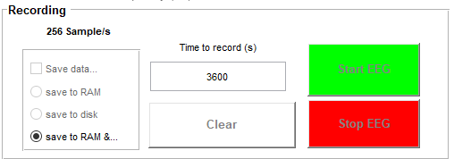
Image 10: The Clear/Start/Stop menu of the EEG_Recorder.
The ‘Time to record (s)’ marks the predetermined recording time.
- Default = 3600 seconds, 1 hour before the recording stops automatically.
- Then acquisition stops and you can save the data.
- However, you can also stop the recording on your own time. (see below: Stop EEG).
- Note: sample frequency = 256 samples/s
- CLEAR: Before starting a new recording CLEAR clears the buffer (your temporary datastorage) and the screen. Your settings remain.
- BEWARE: Never use CLEAR when you havent saved the data: You loose everything.
- Start EEG: Acquisition starts.
- BEWARE: Be patient. It takes a while (seconds) before the signal actually appears on the screen and the green LED on the MOBILab light up continuously.
- The recording stops automatically when the ’Duration acquisition’-time is reached.
- The entire recording of all 8 channels (also the ones that are not connected) are presented on the screen
- SAVE the data: File > Save.
- BEWARE: Not saved is all data gone! So dont hesitate: SAVE the data. After that you have time to discuss, talk, get coffee etc etc.
- Stop EEG: When you want to stop the recording at your own free will, before the ‘Duration acquisition’ is reached.
- BEWARE: Be patient. It takes a while (seconds) before the recording actually stops. Only when the entire recording of all 8 channels appears on the screen, it is ready to be saved. Wait for it before doing anything else.
- SAVE de data: File - Save, in the folder that is automatically opened, the data folder.
- Save to Ram & ... is the default and does not need changing.
TESTING your SIGNAL :
Now you are ready to start your first test recording
Maak eerst vraag II.5 van de Module II Quiz: Motoriekpracticum module II: De eerste EEG meting
- Turn ON the GAMMABox. A green light signals a full battery
- Turn ON the MOBILAB. The LED flashes green when sufficient battery power, and turn red when it needs battery replacement
- CLEAR the buffer
- START the recording
Observe the signal. Discuss the signal quality with the assistent.
If it looks like the image above, you have a clear and clean signal
If it looks like a mess: Trouble shoot!!. A bad signal is usually originating from a bad ground or reference signal which can be identified by a large 50 Hz peak in the FFT plot in the FFT panel. However, also other events can lead to a messy signal.
Adjust until you are satisfied with tghe signal quality. The 50 Hz peak should be barely visible and a stable recording apparent.
Now stop the recording and reset the EEG_Recorder (Press Clear, that is if you dont want to save)
Click image to Trouble shoot, if necessary. A new trouble shoot window will open

THE FIRST RECORDING.
First have a look at both EMG signals
- Start a new recording
- Evaluate the signaal. Still OKAY?
- Ask the test subject to move the wrist up and down, in alternation.
- Observe the signal and discuss the results.
- Now ask the test subject to make a fist with maximum force.
- Observe the signal and discuss the results.
Maak nu vraag II.6, II.7, II.8 en II.9 van de Module II Quiz: Motoriekpracticum module II: De eerste EEG meting
Stop the recording, the program processes the data and wait for the results to be printed to the screen. This might take a while: BE PATIENT!
SAVE the data: File > > Save, in the designated folder. Never use the name of the test subject in your filename, but use a clear anonymus clear name followed by a short description of the experiment: ‘ppn1_arm1’. Never use spaces or strange characters in the name. Onky use letters, numbers and underscores(_)
Reset the EEG_recorder AFTER saving.
Now have a look at the ECG signal
- Start a new recording
- Evaluate the signal: Still Okay, no 50 Hz?
- The ECG signal is best when the left arm rests on the table.
Maak nu vraag II.10 van de Module II Quiz: Motoriekpracticum module II: De eerste EEG meting
Stop the recording, the program processes the data and wait for the results to be printed to the screen. This might take a while: BE PATIENT!
SAVE the data: File > > Save, in the designated folder. Never use the name of the test subject in your filename, but use a clear anonymus clear name followed by a short description of the experiment: ‘ppn1_arm1’. Never use spaces or strange characters in the name. Onky use letters, numbers and underscores(_)
Reset the EEG_recorder AFTER saving.
Nuow its time to focus on the PFC electrode
- Start a new recording
- Evaluate the signal.
- Ask the test subject to sit up and look ahead.
- Observe the signal
- Ask the test person to blink 5 times in a row.
- Observe the results and discuss.
- You recorded a EOG, an electro oculo gram.
Maak nu vraag II.11 en II.12 van de Module II Quiz: Motoriekpracticum module II: De eerste EEG meting
Stop the recording and wait for the data to be processed and printed to the screen. Again: BE PATIENT!
SAVE the data: File > > Save.
Reset the EEG_recorder.
You have finished Module II. he rest of the modules will be dealt with in the sensorimotor practical
You have recorded EMGs ECGs as well as EEG. In Module III you are going to use this in a actual sensori-motor experiment
Fysieke Stress Experiment
Nu wordt het eindelijk tijd om een echt experiment met een vraag en hypothese uit te voeren. Tijdens het uittesten van alle signalen hebben jullie kennis gemaakt met de fysiologische metingen van spieren, en aan het eind ook oogknippers en hartslag gemeten. Nu willen we onderzoeken hoe de spierpotentialen veranderen als een spier vermoeid raakt en of het vermoeid raken van een spier een fysieke stressrespons opwekt bij de proefpersoon.
Dit experiment wordt uitgevoerd door één deelnemer van de groep
Extra materiaal:
- 1 tennisbal of gebruik de geltube om in te knijpen
De electrodeconfiguratie is zoals tijdens het testen van de signalen.
Sluit een proefpersoon aan!
Test nu eerst het signaal
- Start de EEG_recorder weer op (zoals eerder)
- Maak eerst het signaal zoveel mogelijk storingsvrij (trouble shoot als nodig).
- Het signaal moet er ongeveer uitzien als in afbeelding 11, met een extra spierkanaal.
- Als het signaal naar tevredenheid is stop dan de meting, CLEAR de buffer en het scherm.
Afbeelding 11: Zoals de meting eruit kan zien. Hier kanaal 1: hartslag, Kanaal 2: EMG en kanaal 3: Frontaal met Oogknippers
Doe nu het feitelijke experiment
Geef nu de proefpersoon de tennisbal of de geltube in de rechterhand. Laat de tube op de tafel staan en knijp de tube losjes tussen de wijsvinger en de duim. Hou de andere vingers in een vuist. Laat de proefpersoon nu naar een leeg/wit scherm naar de in het midden geplaatste cursor kijken om oogbewegingen zoveel mogelijk te voorkomen en verstoringen te vermijden.
- Start een nieuwe meting met een duur van 1 uur .
- Wacht eerst minimaal 60 seconden voor een stabiele ‘baseline’, zonder de tube al in te knijpen.
- Laat vervolgens de proefpersoon zo hard mogelijk in de tube knijpen en dit 5 minuten volhouden (dus houd de tijd bij).
- Niet even loslaten maar continue blijven knijpen.
- Ontspan na 5 minuten, of eerder als de proefpersoon niet meer kan, maar hou de tube nog wel lichtjes vast.
- Meet nadat de proefpersoon gestopt is met samenknijpen nog minimaal één minuut door.
- Daarna wederom knijpen maar nu elke minuut even loslaten en meteen weer knijpen.
- Laat de proefpersoon dat 5 keer herhalen
- Meet uiteindelijk nog minimaal één minuut door.
- Stop de meting.
- SAVE de data!
- Overleg even met je assistent of er nog tijd is om dit experiment te herhalen met andere personen in de groep.
- Deze data gaan we analyseren in de eerste laptop werkgroep.
- Zorg daarom dat iedereen in de groep de data heeft!
Module III: The sensori-motor experiment
Timing of muscle potentials
In the previous modules you have recorded the muscle potentials and observed that the amount of force that a muscle produces is represented by the amplitude of the muscle potential. In addition to the muscle force, also the timing of muscle potentials is essential to properly perform a task. Because muscle potential recordings are noisy and variable, it is hard to estimate the timing of a single muscle in relation to the action. Therefor we need repeated, timed measurements that we can use to average.
Evoked Related Potentials (ERPs)
The rationale is that noise is random whereas the timed ERP is linked to the action and should be visible in every trial. By averaging the signal on the basis of the action noise is cancelled out and the ERP becomes visible. Also the ERPs so often presented in papers concerning cognition research are constructed in this way. Here you will perform an ERP experiment: The muscle potentials of the muscles that are used to press a key on the keyboard will be recorded. But that is not all! The activity of the frontal cortex, the motor cortex and the parietal cortex will be recorded simultaneaously. In this way you can study the timimg between activation of the cortici, the muscle potential and the actual keypress.
The experiment is a replication of a paper by Nieuwenhuis 2003. In short: test subjects are presented with high and low tones and react to them according the instructions. In fact this is a Go-NoGo task!
The experiment is performed by one member of the group. Preferably some else than in the previous recording
Now we are going to use the full setup that is place in front of you; Materials:
- Two laptops (Recording and stimulation laptop)
- Five recording elektrodes, and one ground and one reference electrode
- Recording equipment
- EEG-gel, elektrode stickers, tape
STIMULUS COMPUTER
To record the key-presses and couple them to the muscle potentials we use a Matlab Go-NoGo program that has been made especially for this practical 'GoNoGo.m' that is present on the stimulus computer
.The Experimental setup and what the task sends to the EEG_recorder
- The onset of each and every tone is detected and passsed to the EEG recorder
- The onset and identity of every keypress is detected and passsed to the EEG recorder
Logging the events
- All events of your choice are transferred to digital pulses
- These pulses are send to the Digital Input/Output (DIO) box (National Instruments: USB-6501)
- The marker (TTL) is send to the EEG-recording laptop via a predetermined (by the task developer) gate on the USB-6501.
- TTL, short for Transistor-Transistor Logic is a standard digital pulse for communication between electronic equipment and circuits
- The receiver reads the signaal (0= maximum 0.8 Volt, 1 = minimal 2.0 Volt).
- In this experiment, the markers indicate the onset of the keypresses and tones as recoded by the task laptop.
- The analysis software, as part of the EEG_recorder program, can cut the EEG according to the markers and produce ERPs.
- The individual ERPs can be averaged into a proper ERP related to a particular event.
Of course the ERPs only make sense if controlled by a proper task that delivers meaningful stimuli.
For now, the GoNoGo experiment is up and running and preprogrammed. However, you have to design your own task that suits your own experiment.
LOADING AND SETUP OF THE BEHAVIORAL TASK
- Download the GoNoGo folder from CANVAS and unzip on the desktop.
- Start MATLAB 64-bits.
- Make The GoNoGo folder your Current Directory in MATLAB
- Double click the GoNoGo.m file, it opens in the editor.
- Now first read through the code and notice what it does.
RECEIVING MARKERS IN YOUR EEG-RECORDING
Each time a key is pressed and a tone is played on the task laptop, TTL pulses are send to the EEG recording laptop via the USB-6501. Only when the EEG recording laptop is set to receive, the markers will actually be stored with the EEG recording (Picture 13).

Picture 13: TTL-puls panel in EEG_recorder. Select the markers that have beeen set in the task laptop. In the sensori-motor experiment you need all six .
Test the connection of the task laptop with the recording laptop
Before you perform the experiment it is essential that you test whether everything is set up properly. You van do this by performing a marker test
Selecteer op de stimulus laptop de Marker test!.
- Start MATLAB 64-bits on the task laptop.
- Open the script Test_Markers_NI_USB_6501.m in the editor (double click).
- Have a look at the script and try to get an idea what it is going to do
- Start the EEG-Recorder without connecting a test subject
- Now run the script.
- The command line of MATLAB shows the progress.
- The connection with the USB6501 is configured and the marker channels are loaded.
- Watch the EEG-recorder recording and verify that it is doing what you already figured out.
The Marker test program stops automatically.
STOP the EEG_Recorder and SAVE the file
Now observe the saved file, that is still visible in your recording window.
Verify that the markers are actually recorded by the EEG_recorder.
Maak Vraag III.4 van de Module III Quiz: het sensori-motor experiment
In case of a succesfull marker test, the real sensori-motor experiment can start
Make The GoNoGo folder your Current Directory in MATLAB
Double click the GoNoGo.m file, it opens in the editor.
Get the EEG-Cap, call one of the teachers and have them explain how to place the electrodes
Maak Vraag III.5 van de Module III Quiz: het sensori-motor experiment
Choose a new test subject.
- Three red EEG electrodes are connected
- Place at locations FZ, C3 and PZ
- Yellow ground on CZ
- Place the EEG cap on the head of the subject.
- Measure Inion and Nasion (see image 14) and fit the cap in line with the international standard, the 10-20 system.
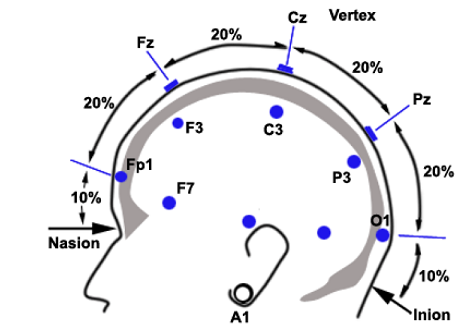
Image 14: Left the location of CZ elektrode with reference to Nasion and Inion. On the right the standardized placements of electrodes.
- Place electrode 4 on the Digitorum extensor
- Place electrode 5 op the Palmaris longus
- Fix the wires with some tape to release the pressure on the electrode.
- Clip the reference electrode on the earlobe.
- The yellow ground is now placed in the Cap on Cz
- Gel all electrodes (See Image 15)
Afbeelding 15: Het ‘gellen’ van de elektrodes.
- Run the EEG_Recorder while stabilizing your signal.
- A proper ERP depends on the quality of your signal.
Vul tabel bij vraag III.6 in van de Module III Quiz: het sensori-motor experiment
Now, write your logbook with all the settings
Prepare the EEG-Recorder
- One of your team is responsible for the recording during the experiment
- Switch ON EEG channel 1 through 5
- Switch On all six marker channels
- Start The EEG_recorder.
- Check the signal.
- Adapt if neccesary.
- Stop, clear and start the EEG_recorder again
Start the Go-NoGo task on the Task Laptop.
- One of your team is responsible for everything concerning your test subject during the entire experiment
- Run the Go-NoGo task
- The connection with the USB-6501 is made and the marker channels initiated.
- The experiment starts running
The experiment runs for about 20 minutes.
- Stop your EEG recording
- BE PATIENT: Wait for the download of the buffer to the screen, this can take sime time after a long experiment
- NOW, SAVE YOUR DATA, immediately. Save first, discuss later.
- KEEP AWAY from the CLEAR BUTTON AF!.
Release your test subject
Copy all the recording files to every member of the team.
NOTE: You can't email .mat files. These are considered virus susceptable. You need to zip the files before distributing.
- The recording file is located on the EEG-Recorder Laptop
- In the folder where you saved the file.
- Most probably in the data folder of the EEG_Recorder program on the desktop
- De behavioral file with the identity of the key presses etc etc is on your task laptop
ANALYSIS TIME
The analysis by the team
Module IV: The analysis of the EMG signals
All data is stored so its analysis time
Here we focus on the analysis of the EMG signals. The analysis of the EEG recordings follows similar steps, however, not all parameters are the same so think before you do!
Als je onderstaande stappen hebt doorlopen en begrepen, verwijzen we voor de analyse van het EEG in relatie tot de tonen naar de ERP_ANALYSIS pagina. Daar staat meer uitleg over het hoe en waarom
Loop nu onder de stappen door om het EMG te analyseren.
DATA ANALYSIS in 6 logical steps
Data analysis usually is performed in a few logical steps.
- Filter out unwanted frequencies in your data
- Cutting the data on the basis of the marker onsets: create individual ERPs
- Baseline correction to 'zero' the baseline of individual ERPs
- Select relevant ERPs
- Average the cut and corrected ERPs
- Visualization of the averaged ERPs
Below each step is dealt with in order.
STEP 1: FILTER OUT UNWANTED SIGNALS (FREQUENCIES)
the datafile that you have just recorded and saved is what we call 'Rough data', 'Ruwe' data in Dutch. The largest disturbance in the signal is the 50 Hz noise from the electrical grid.
So we have to delete them by using the filter tool.
Unwanted frequencies in the signal can be filtered out in Four ways.
- Low-pass filtering All frequencies lower than a set value remain in the signal
- High-pass filtering All frequencies higher than a set value remain in the signal
- Band-pass filtering All frequencies between two set frequencies remain in the signal
- Band-stop filtering All frequencies between two set frequencies are taken out of the signal
To remove the 50 Hz artifact we are going to use a band-pass filter with boundaries of 0.05 and 48 Hz.
BEWARE: in an EMG signaal high frequencies are not important, however, if you are interested in the high frequenties in your data such as gamma oscillations, you might want to use another method to get rid of the 50 Hz.
Discuss with your group what the procedure would be if you would like to keep the gamma frequencies.
- Open The filtertool
- Load your original 'rough' data file
- Check: apply filter to channels: First 8
- In this way you don't filter the channels with the markers
- Check: band-pass filter
- Filter between 0.05 and 48 Hz
- Do not Check: Plot results
- Filter
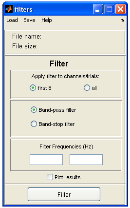
Image : Filter Tool. for applying, band-pass and band stop filters and Power analysis.
This results in two save windows, The first one saves the complete filtered data. Thats what we need. The second one calculates one power value for the entire file. You can cancel that one. If we would want a power analysis, we will use the 'TF_analyse' tool in EEG_recorder
The data is now free of 50 Hz.
STEP 2: CUTTING THE DATA
The second step is to cut the data in short segments on the basis of the onset of the keypresses. The tool for this is the ‘Event cutter’.
- Open ‘Event cutter’ in the EEG_recorder tools. It looks like the image below
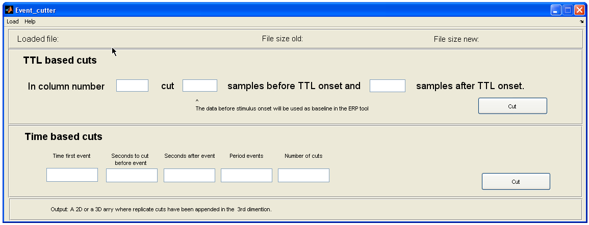
Image : Event cutter Tool. Used to cut EEG data in ERP segments on the basis of marker events.
Each time a key is pressed a TTL-pulse is send to the recording laptop (the DIO's or markers). We would like to cut the data based on these TTL-marker pulses. Therefor you have to load the data first, the filtered data file that you have just created.
- Load the data: File -- load.
We are using the 'TTL Based cuts' section. The TTL-pulses of the keyboard and the onset of the tones are saved in channels 9 - 14. The first eight are always your EEG channels and then one extra channel for each marker channel. So you have a maximum of 14 channels (8 EEG/EMG channels and 6 marker channels).
If the sensori-motor experiment is properly executed, you actually have data on all 6 marker channels. Have a look at the explanation of the Go-NoGo task what is actually recorded.
Discuss with your group why it would be wise to use the marker channel 6 (= recorded channel 14) if you are interested in the EMG of the keypress.
- Select channel 14, in the experiment this is the channel onto which the keypresses of condition 2 are recorded. In Matlab the data of the individual channels are stored in columns. So file in 14 as column number (see image 16).
We are now first interested in the reaction of the muscles in relation to the keypresses.
Discuss what the time relation is between the reaction of the muscles in relation to the keypress. You might want to set the cut a bit earlier than the onset of the keypress. WHY??
- Therefore, Cut the data 256 samples (1000 ms) before the marker onset and 128 samples (500 ms) after the marker onset. NOTE: The unit here is ‘samples’ (What was the sampling frequency of the EEG system?).
- Press ‘cut’, Now you cut short pieces of data from each EEG channel surrounding the onset of the keypress on the basis of the set parameters.
- Save the data and use the original name with the extension _cut (Never use spaces or signs other than letters, numbers and underscores, Matlab is allergic to that). Save into the datafolder on your desktop.
Before you close the event cutter, have a look at what the cutting procedure actually resulted in: see 'File size new'. There are three numbers there. Determine, with your group what these numbers actually mean.
How many keypresses did you expect? And, does that match with what you see?
STEP 3: BASELINE CORRECTION OF THE ERPs
Now close 'Event_cutter’.
The next step is to correct the baseline for each and every ERP that you have produced. You can use the ERP tool for that (Indeed, you can find ir in the toolbox).
- Open ‘ERP tool’ in the EEG_recorder tools.
- Load the file that you just saved and which houses the ERPs (File -- Load).
- In the green section: The first number represents the amount of samples of each ERP, the second number is the amount of channels. In the (new) third dimension and all the individual ERPs that were just cut. We would like to adjust the baseline for all these ERP sections.
- In the blue section
- Channels to browse: leave that on '1'. The baseline correction is automatically performed on all channels.
- Onset (in sample nr!): provide the length of the baseline. Basically the amount of data before the marker onset.
- Fill in : 256 samples. This is one second with the sample frequency of 256 samples per second
- ONSET in sample nr: 256 samples. This is one second with our sample frequency of 256 samples per second. We hereby take the first second of the each ERP as the baseline or control measurement.
- The principle of baseline correction: We took many 1.5 seconds sections of data from the file. If you consider the fact that there can be a low frequency oscillation with an amplitude of 100 microvolt and a frequenty of 2 Hz runs through your data than some ERPs are cut when the low oscillation is at its peak and some when the low oscillation is in a trouph. The first case the ERP starts at 50 microVolt, in the second at -50 microVolt. The baseline correction takes the average of the amplitude of the first second of each ERP, determines the deviation from the '0' line and corrects the amplitude of the entire ERP with that number.
- Click on Baseline Correction: Each ERP, for every channel is now corrected with there own baseline values.
- Save the data Use the old name with the extention _bl. Save to the datafolder on your desktop.
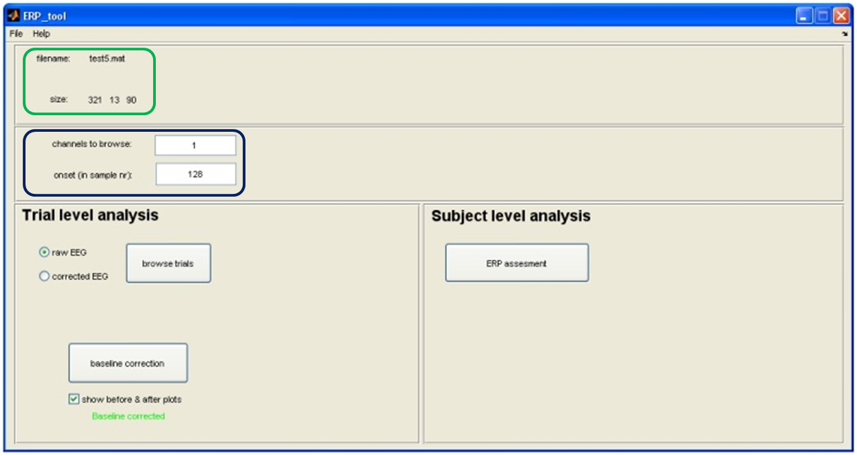
Image : ERP_Tool. For adjusting and analysis of ERPs.
The data is now baseline corrected.
STAP 4: SELECTEREN VAN DE JUISTE MARKERS
THIS STEP IS NOT NECCESSARY FOR THIS ANALYSIS, SO SKIP AND GO TO STEP 5. There are occasions when you are actually going to need this step. For instance, if the markers in a given channel are a mix of various events
De volgende stap is het selecteren van de juiste events binnen de geknipte stukjes EEG data.
NOTE: Na alle tonen werd er ongeacht of er een key wordt ingedrukt een 'keypress' marker gecreëerd. Eigenlijk geeft de marker het 'end of trial' aan. Dus de ERPs die geknipt zijn zijn een mix van werkelijke keypresses EN het aflopen van een trial zonder dat er een keypress heeft plaatsgevonden. Haal uit je gedragsfile (de .csv file) welke markers werkelijk gerelateerd zijn aan een keypress. Deze ga je nu selecteren door de 'end of trial' stukjes data te verwijderen.
- Open ‘Array Manipulator’ in de EEG_recorder onder tools. We gaan nu rechtsonder 'Selection' tool daarvan gebruiken
- Laad eerst de zojuist gemaakte basislijn gecorrigeerde file (File -- Load).
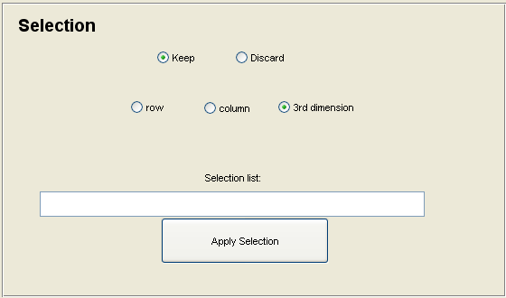
Afbeelding : De selection tool binnen de Array_manipulator_Tool. Voor het selecteren van stukken data uit je file.
De eerste twee dimensies van je dataset zijn meetpunten in de tijd en de verschillende kanalen. In de (nieuwe) derde dimensie zitten de verschillende stukjes die we net hebben geknipt. Hier gaan we nu alleen de werkelijke keypresses selecteren door de 'end of trial' markers te verwijderen.
- Kies daarom ‘Discard’ en ‘3rd dimension’
- Vul nu alle trial nummers in die NIET geleidt hebben tot een keypress, gescheiden door een comma. Dus bv. 1,3,5,18,24
- Click op 'Apply Selection'
- De derde dimensie, links bovenin de 'array manipulator' tool, geeft nu aan hoeveel trials er zijn overgebleven!
- Sla deze data op onder de oude naam_filt_cut_bl met de toevoeging _keypresses (gebruik geen spaties, Matlab kan daar niet tegen). Sla het op in je datafolder op de desktop.
De data bestaat nu alleen uit geselecteerde trails met keypresses.
STEP 5: AVERAGING THE DATA
The next step is averaging the data. For that we are going to use the Array_manipulator (found in the tool box).
- Open ‘Array Manipulator’ in the EEG_recorder tools. We are using the 'Average along dimension' tool
- Load the file with the selected keypresses (File -- Load).
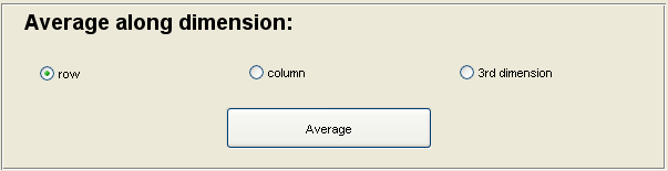
Image : The 'Average along dimension' tool as part of the Array_manipulator_Tool. Use to average data within a file.
The first two dimensions (columns) of the dataset are the data points in time and the different channels. The third dimension hold the various ERPs that have just been baselined. These will now be averaged.
- Choose ‘Average along dimension:’ ‘3rd dimension’ and press ‘Average’.
- The third dimension disappears (is now 1 average).
- The averaging has taken place for all 8 channels. NOTE: So your channels of interest as well as the rest of the channels are averaged.
- Save the data Use the old filename name_filt_cut_bl and add _keypresses_avg (SAgain, no spaces, Matlab doesn't work well with spaces). DSave in the data folder on your desktop.
The data is now averaged over all ERPs.
STEP 6: PLOTTING THE DATA
The result of it all is 8 channels with 1500 ms of dta each: a 1000 ms before and 500 ms after the onset of the keypress.
- Now close ‘array manipulator’.
Now it is finally time to look at the result. Use Data_plotter in the toolbox.
- Open ‘Data plotter’ in the Tools menu
- Load your data_cut_bl_keypresses_avg file.
- Select 'Plot Columns' to plot one average ERPs. Remember that Matlab has stored each channel data in its respective column.
- Set The ‘Onset (s)’ on 1 s (This sets the '0' of the ‘X-axis’ on the time in the ERP that holds the onset of the keypress.
- Note: this 'Onset' setting is completely dependent on the pre marker settings that you chose during the cutting process!!
- Select in 'Rows/Columns to plot', both channels that hold your EMG signals!
- Press ‘Plot’.
- Maximize de plot
- AND?!.......
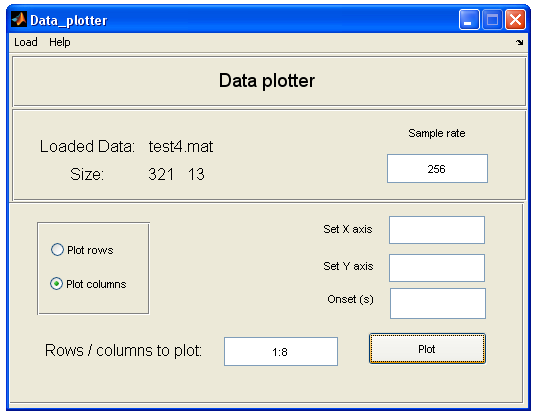
Image : The Plotting tool. To plot your data.
Discuss the result with the group.
- Note: The direction of the response (negatief or positief) doesn't really matter in an EMG plot, its all about when the muscle reacts in relation to the onset of the keypress.
- Is it what you expected?
- Can you distinguish the Flexor from the Extensor?
ERP analysis of the 'audio' data:
Now that you are familiar with the ERP analysis its time to use the ERP analysis pipeline to analyse the Audio triggered results from the three EEG channels.
Devide the group in two, one group performs the analysis of the GO data, the other the No_Go data
Use the ERP Analysis pipeline on the ERP ANALYSIS PAGE (link below).
Here you find additional information on the procedures that you just used
For the analysis of EEG ERPs it is neccessary to look at each and every individual ERP before you attually include them into the average. Only when they are artifact free, include them.
This procedure is called 'Artifact Detection'
Now plot the GO and the NoGo ERP for all three channels
Compare the responses within each condition and between each condition