Analysis of Event Related Potentials: Step by Step
by Dr. Hannie van Hooff & Dr. Tonny Mulder

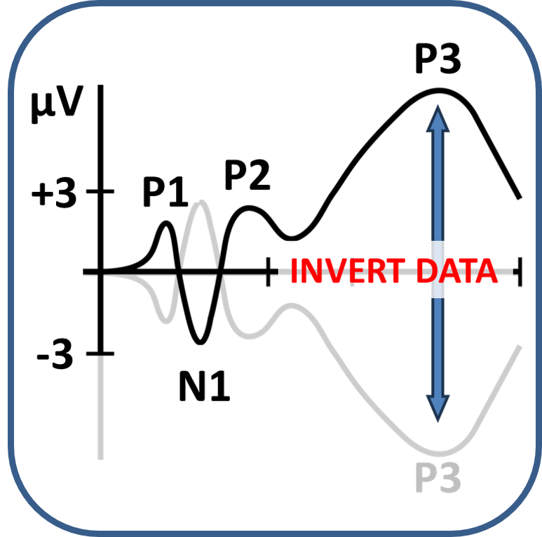
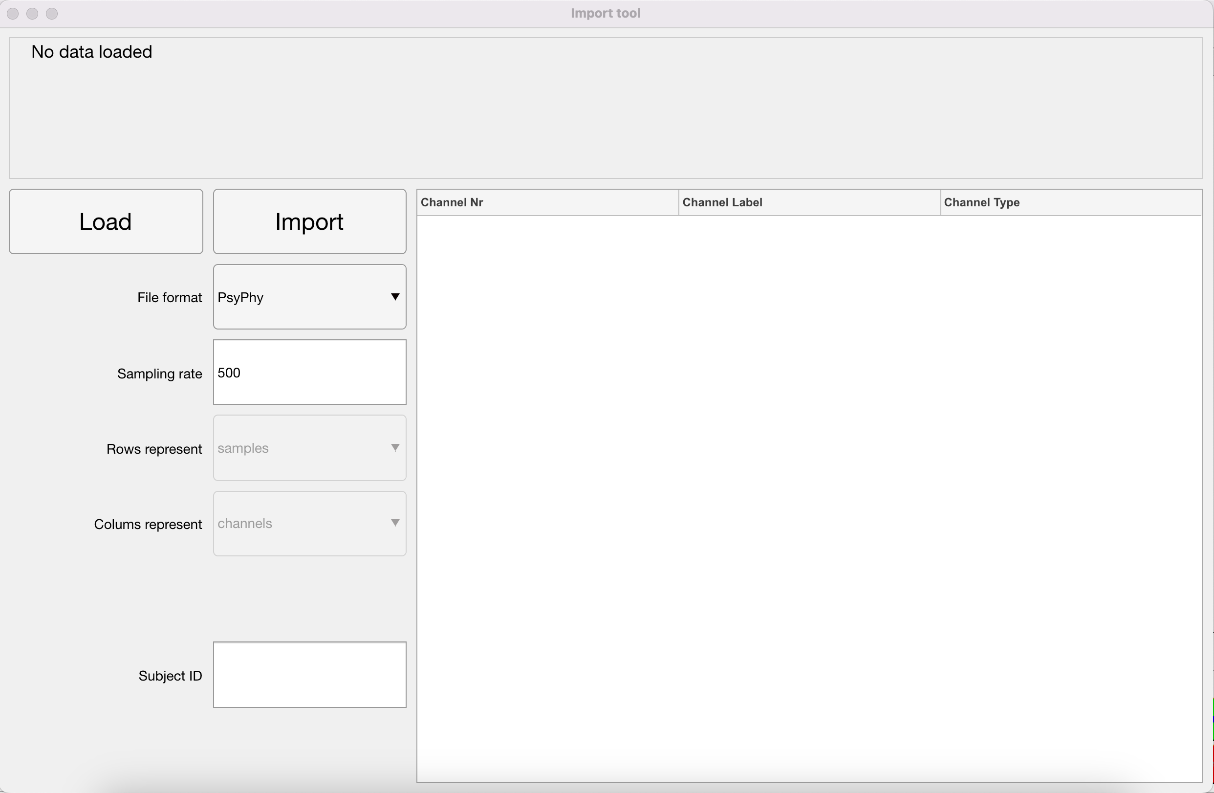
Importing (and Inverting) Data
First things first, before you can analyse the data, you have to import the .mat file created after the PsyPhy recording stopped for use in your MATLAB environment. In addition, as you might have seen by reading EEG papers, the standard in EEG data collection is still that positive waves go down and negative waves go up. Also the PsyPhy system is wired like that. In recent years, researchers tend to correct that. So for now, by importing the .mat file, the data in the resulting imported file is inverted. Positive waves, like the P300, go up and negative waves, like the N400, go down. You will also notice that the eyeblink artifacts that are prominent at frontal recording sites have now switched to positive waves.
Inverting Data
SKIP THIS STEP: If your file has already been imported via the import function above, your data has already been inverted.
As you might have seen by reading EEG papers, the standard in EEG data collection is still that positive waves go down and negative waves go up. Also the PsyPhy system is wired like that. In recent years, researchers tend to correct that. So for now you have to invert the data of your .mat file so that positive waves, like the P300, go up and negative waves, like the N400, go down. You will also notice that the eyeblink artifacts that are prominent in frontal recording have now switched to positive waves.
If you need to invert manually follow the procedure below!
Filtering
Tool to use in recorder: Filter
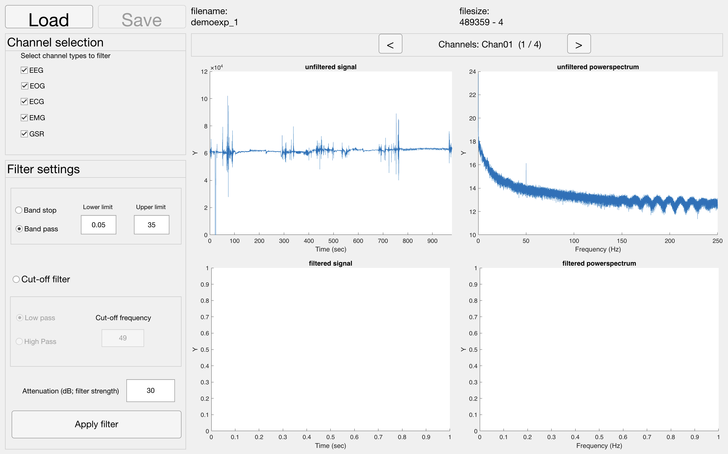
During the recording, your EEG signal can become contaminated by sources other than from the brain, such as the mains grid (our electricity network. This produces a high-amplitude 50 Hz artifact (60 Hz in the USA), often ‘repeated’ at the multiples of the frequency (at 100 Hz, 150 Hz and so on). It is important to filter this artifact out by using a notch filter (which filters out only one frequency) or a band-stop filter (which filters out a frequency range, e.g. 48-52 Hz).
Alternatively, if you are not interested in high frequency EEG data at all (and for ERP research that is most often the case) you can use a lowpass filter of 40 Hz (apart from 50 Hz noise this also filters out activity related to muscle tension). In addition, to exclude very slow activity (for example due to perspiration) you could combine this with a highpass filter of around 0.1 Hz. This low-pass and high-pass filter combination makes a band-pass filter of 0.1 - 40 Hz.
Beware
In principle you are free to choose your own filter settings, but make sure you do not throw away the signal of interest. For example, what frequency do you think the LPP has or the CNV? These are low frequency signals and you need to set your highpass filter well below the frequency of these ERPs.
NOTE: If no signal or powerspectrum appears, go back to matlab. You probably have an error along the lines of "you don't have the Signal Processing Toolbox". Download this toolbox by clicking on the error, and try again.
Epoching data or Cutting.
Tool to use in recorder: Cutting tool
NOTE: Please note that you need a baseline period before the stimulus onset and you have to allow ample time after the stimulus onset to allow for a full ERP to develop. So, specify how many samples (milliseceonds) you are going to cut before and how many after the event onset.
The continuous EEG data file you have recorded contains multiple events.
In this step you are going to indicate which segments (or epochs) of the EEG you want to keep for the averaging process, i.e., the EEG surrounding the events of interest. Thus, you are going to divide/cut/epoch the EEG into smaller segments, often referred to as “trials” (see figure on the right). For sensory ERPs, make sure you also include some EEG that precedes the stimulus presentation, so that you can use this as a baseline (typically 200-250 ms). The part following the stimulus event should contain all components of interests in full, including the return to baseline. A typical post-stimulus period is 1000 ms.
Once your EEG signal is segmented into trials, it will have changed from a two-dimensional data set (samples x channels) to a three-dimensional data set (samples x channels x trials). By looking at these 3 dimensions, you can check whether the segmentation was performed correctly. The number of samples (first dimension) should correspond to the time period between the cutting margins you chose. If you know the sample rate of your recording (in our experiments it will most likely be 500 samples/second), you can calculate samples to seconds and vice versa. The number of trials (third dimension) should correspond to the number of events (markers or triggers) you send out from .
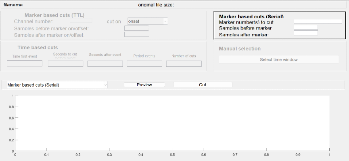
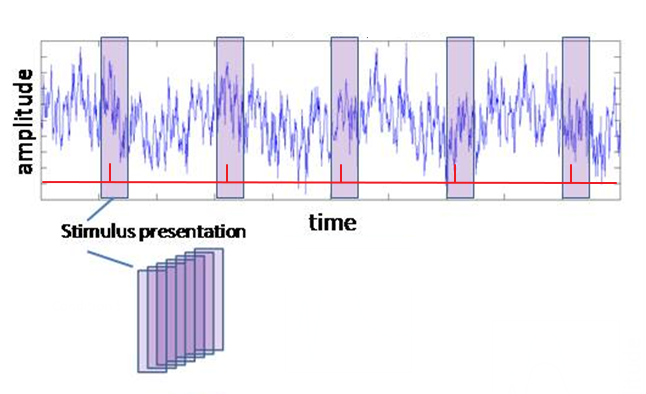
Figure: Segmenting the raw recording into individual trials. On the basis of your triggers (in red) select designated sections from your data and stack them.
Baseline Correction.
Tool to use in recorder: ERP-Tool: Baseline correction
Commonly, the size of an ERP is measured relative to a baseline defined by the pre-event period. An assumption of this method is that baseline values are similar across subjects and conditions. To meet this requirement, we need to perform a baseline correction: for each trial, the mean value of the baseline period is calculated and then subtracted from the pre-event and the post-event parts of the signal. In this way, the mean baseline value of every trial is set to zero so that the segments can be averaged and compared.
NOTE: Don't forget to set your 'onset value', before applying baseline correction. It sets your event onset and thereby the 'pre-event' time. You can get your onset value by remembering what the 'Samples before marker' where while cutting the ERPs.
No need to set 'channels to browse' since it will perform the baseline correction for all channels simultaneously
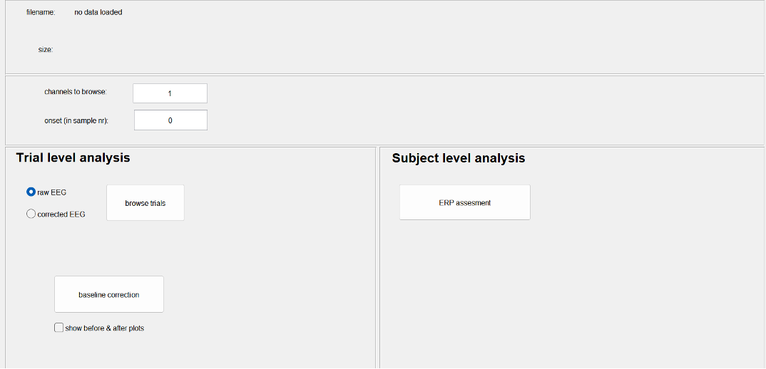
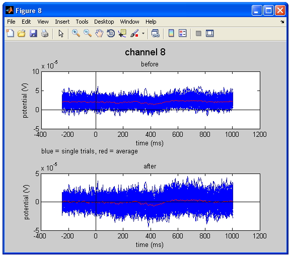
Figure Baseline correction. The upper figure represents the raw data, whereas the lower figure shows the baseline corrected data. Note that the average of all trails in the plot (the red line) shifts towards 0 V in the corrected data.
Artifact Detection.
Artifact Detection.
Even after filtering and baseline correction, your EEG signal may contain artifacts such as muscle activity, eye blinks and other movement artifacts. A simple method to remove these artifacts is to inspect each trial visually and reject trials that look contaminated. This can be very time consuming but it offers a lot of control over the cleaning process and more insight into the nature of your signal. To save time within the context of your experiment, you can decide to perform this step (and the next ones) for a selected set of channels only.
Because the criteria for rejection are arbitrary, you are advised to start working in pairs so that you can define “rules” for yourself, and make these explicit! For that purpose it is also good to look at papers to see what criteria they have used in their automatic artifact detection procedure (see my example above). In principle these criteria should be reported but not all researchers do so + this also depends on the specific journal.
Making use of the standard deviation
There are several ways to detect artifact. A useful criterion could be that each individual EEG trial should fall in between 2 to 3 SD of the average. But, as the examples of the Figure on the right how you, there will still be many ambiguous cases. Please also check the values of the Y axis, because the program automatically adjusts these to the highest value within that particular data set. You thus could end up with very different max-min values for individual participants. In addition, to give you some idea of scale, note that the scale for EEG (often ± 100 µV) is very different to that of an ERP (often ± 10 µV). A difficulty is that you should not end up with too few trials to be able to calculate a reliable ERP. Remember that you need at least 25-30 trials for a reliable P3.
The best way to keep rejection levels low is to prevent them from happening!
Thus, make sure electrodes are well connected and ask your participant to relax their muscles, and to move or blink as little as possible.
Selection of artifacts.
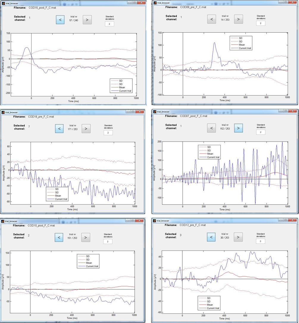
Figure: Examples of EEG trials that exceed the 2 Standard Deviation (SD) limit. Some cases however are more “disturbing” for the calculation of ERPs than others. Can you figure out which ones?
Sorting by condition/Artifact Deletion
NOTE: Only use this tool if you forgot to add specific markers and your markers have no label!!
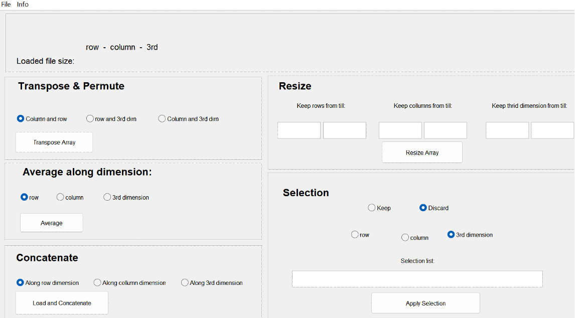
Tool to use in recorder: Array manipulator: Selection
Before averaging, you need to sort the trials by condition and save the data for each participant/channel/condition as separate files. The idea is to create new files containing the trials for each condition and each channel separately. As mentioned before you should do this for the artifact-free trials only. So exclude the ones you marked as containing an artifact (see artifact detection section). This will result in a large number of files, therefore it is important that you carefully document and that you use clear anonymous file names (e.g. subj2_filtered_cut_cond1_Fz, proefpersoon3_O2_cleaned_neutral,). Do not use dots or spaces or special characters in the filename except for the .mat extension, for this can lead to loss of data!
IMPORTANT: don't forget to reload the same baseline corrected dataset before selecting another channel of the same condition!
Averaging.
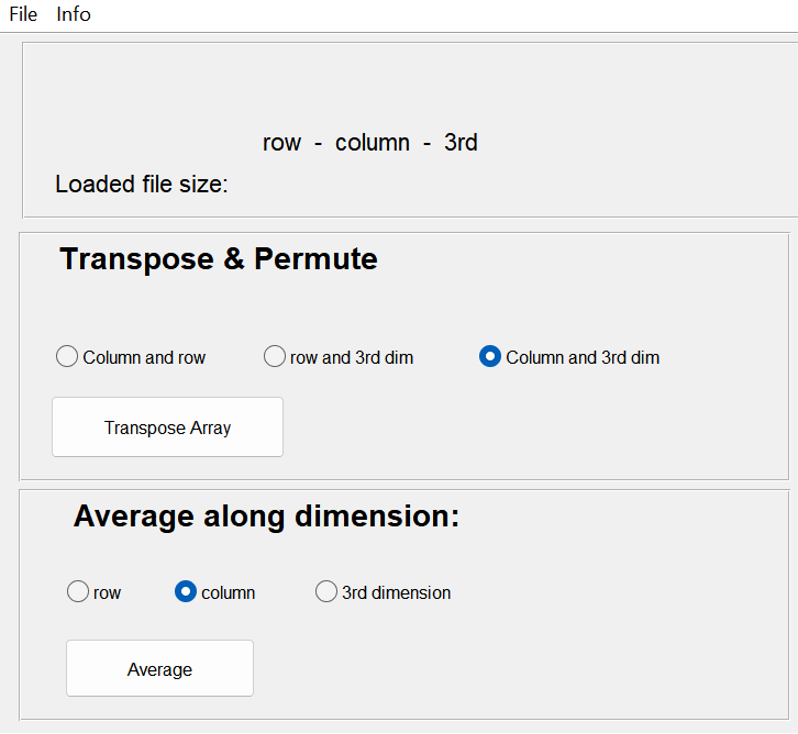
Tool to use in recorder: Array manipulator: Averaging
Next, you can create an ERP by averaging all trials for each participant, channel and condition. Make sure that you average in the correct dimension of trials. For example, if you are processing one channel each time, the dimensions may have switched.
Don’t forget to save a new file for each average/ERP you created and to give it an appropriate name.
Merging Participants.
Tool to use in recorder: Array manipulator: Concatenate
For the statistical analysis you will use the ERP data per participant, but you can now already plot the ‘grand average’, which consists of the mean ERP of all participants together. The grand average plot can be used to see if the ERP is present and to check if there is a visible difference between your conditions. To do this, you need to merge the files of each participant in one larger file for each channel and condition separately. This is called ‘concatenating’ of the files. The result should be a number of files (as many as channels x conditions you have), with the samples in the first dimension and the participants in the second dimension.
Making use of the standard deviation
You could then plot (for each channel and condition) the grand average ERP of all the participants. The most useful is to plot for each channel separately the grand averages of all conditions. Thus, for example, for electrode position Pz, you plot ERPs for condition A, B, and C. In this way, you could easily compare (within one graph) between conditions. You can also use these graphs to determine the time window and channel location at which your ERP effect is the strongest. This time window is important for the calculation of the ERP size later on (see next step). Generally, the grand average for all conditions (per channel) is also the graph that you would like to show during your presentation to underline your results.
Example.
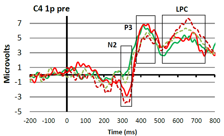
Figure: ...
Measuring the Amplitudes in your ERP
Tool to use in recorder: ERP Tool: Subject level analysis
HELP: ERP Amplitude Tool
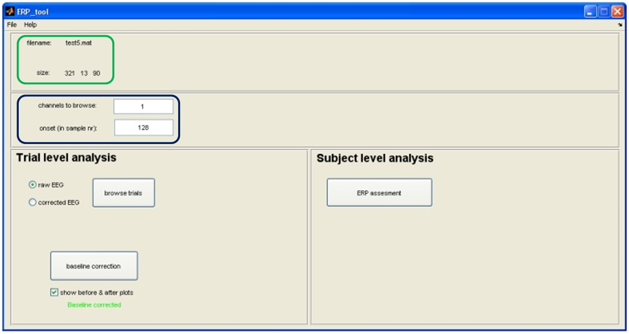
ERP-Tool window
The top panel in green: name and size of loaded data set.
In the second panel in blue: select the channels you want to view. Note that the trial browser allows you to view multiple channels at the same time, while the ERP assessment can only view one channel at a time.
In the “onset” field: Baseline time before event in samples(the number of pre-event samples you defined in the Event Cutter tool).
Subject level analysis
Assess the measures of ERPs when they have been averaged per subject.
Use after baseline correction AND after artifact rejection
Browse Trials
It allows you to:
- Scroll through the ERPs of different subjects
- Select a time window around your ERP component of interest
Get information about:
- The peak amplitude (for positive and negative peaks)
- The peak timing (for positive and negative peaks)
- The average amplitude
- The area under the curve
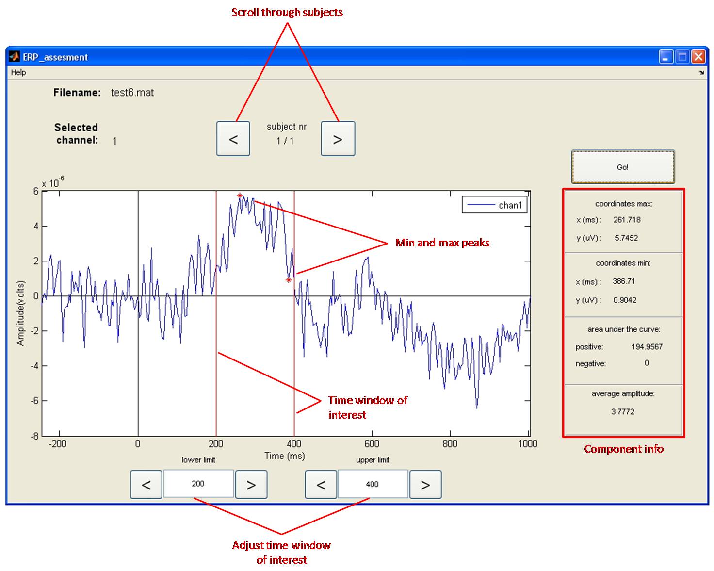
Fill in a lower and upper limit in milliseconds of your time window of interest. Click “Go!” and two red lines are drawn indicating indicating the lower and upper limits, two red stars indicate the location of the min and max values within the limits, and the bar on the right side displays the measures of the selected component. Write down the values you are using for your analysis and repeat this for all subjects.
For statistical analyses (for example to answer the question whether the observed ERP amplitude difference is significant or not?) one has to quantify the individual ERPs. There are several methods to do so, which will be described next. Please note, we illustrate this with reference to grand-average waveforms while the software will do this on the individual ERP waveforms, which are a lot more ambiguous due to individual variation!
Peak to baseline method
the peak-to-baseline method, comes down to measuring the maximum value of the ERP (or minimum value for negative components) with respect to the pre-stimulus baseline (which is set to 0). Alternatively, you can measure the peak-to-peak-value, which is the distance from the maximum value of a positive component to the minimum value of the following negative component, or the opposite. For these methods to work, there needs to be a clear peak in the individual waveforms, which typically is only the case for the early components (like P1 and N1). A potential disadvantage of this amplitude measurement is that peak measures are very sensitive to the presence of background noise.
Example peak to baseline analysis.
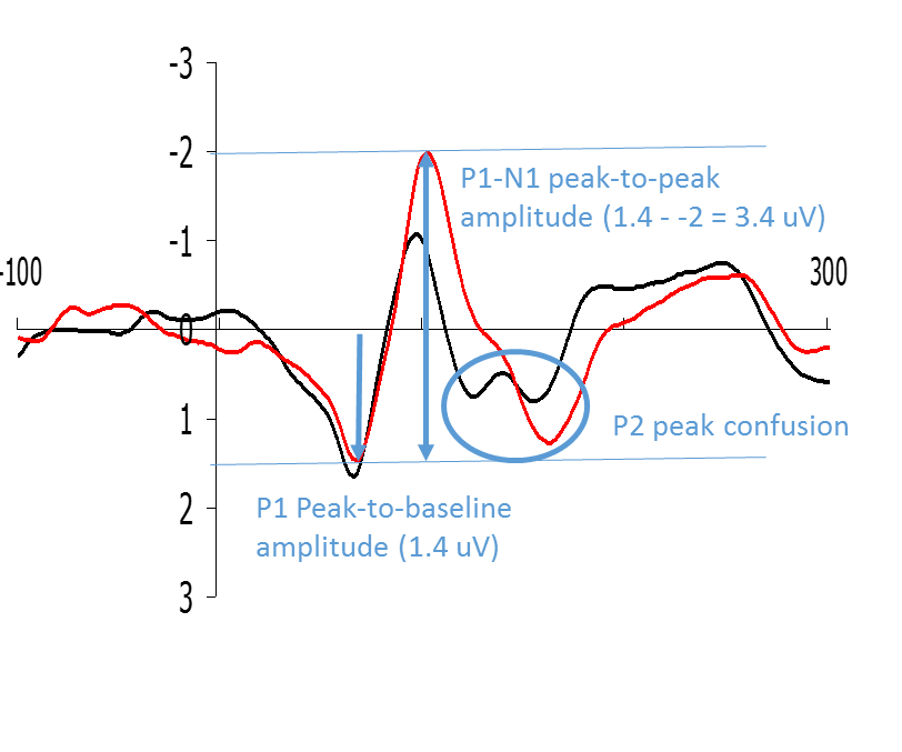
Figure: Examples of how P1 and N1 can be quantified by means of peak-to-baseline and peak-to-peak measurements respectively.
'Mean Amplitude in time window' Method
The peak-to-baseline or peak-to-peak value is not always a good representation of the size of the ERP, especially in the case of late components. The peaks of these late components are less sharp or are spread out in time, and sometimes they drift upon each other. In other instances, like in the figure, it is not clear exactly which peak to take. In these cases, it is better to measure the mean amplitude of a certain time window (Figure).
The setting of time windows for finding peak values (max or min values) or for calculating mean amplitudes is a tricky business. This is because peaks and waves do not always appear around exactly the same time across experiments and across electrode positions. You should select a time window based on (1) what can be seen in the grand-average, and (2) what has been reported in the literature (see citation below from Keil et al., 2014). Many students have difficulty with this method as it feels biased and subjective, and in a way it is! On the other hand, it makes no sense to set a time window purely based on your expectations of a particular component (say a P300 window of 200-400 ms) when in your actual data no positive component is present at around that time. To avoid ambiguities in your report, describe precisely how you tackled this problem.
Example mean amplitude analysis.
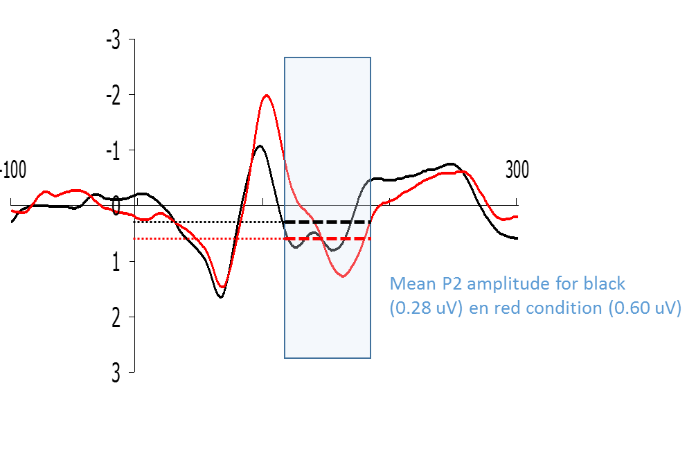
Figure: Example of how a P2-type wave could be quantified by means of calculating the mean amplitude of a certain time window.
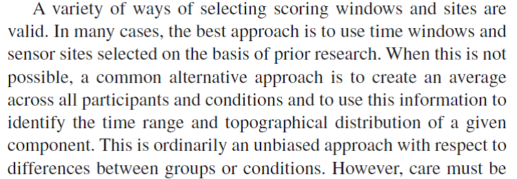
Figure: Citation about selecting scoring windows from Keil et al. (2014)
Super Grand Average
In the figure, you can see how the advice mentioned in the citation above works in practice. At the top you see a super-average waveform calculated by averaging all conditions and channels together (in this case 4 conditions and 2 channels/electrode positions). Based on this waveform, you can set time windows for the different peaks and waves that are of interest in your experiment (in this case N2, P3, and LPC). This is reasonably objective because in this way you are not influenced by ERP amplitude differences that are visible when looking at the averages of each condition plotted over each other (see bottom Figure 8) (please note, personally I think that the P3 time window in this case could have moved 30 ms to the right). Once you have decided which time window you are going to use to quantify a certain ERP peak or wave, you have to go back to your individual ERPs. For each individual participant and each condition you apply the agreed measurement method. So for example, in the study that produced Figure 8, it was decided to quantify the LPC wave as the mean amplitude in the 520 to 750 ms post-stimulus time interval. Since each individual participant was exposed to two conditions, this means that for each participant two LPC amplitudes will be calculated; one for the dotted line condition and one for the solid line condition. These individual amplitude measures (as indicated in the Table below) will subsequently be used for the statistical analyses.
super grand average
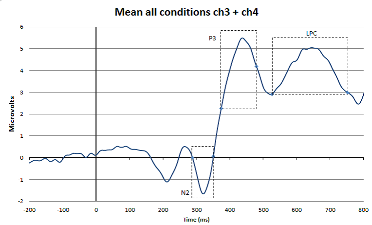
Figure: Top: Example of a super-grand-average in which ERPs were averaged over 4 conditions and 2 channels/electrode positions. This super-grand-average is used, together with relevant literature, to select objective time windows for the ERP peaks and waves of interest. Bottom: Example of how the time windows fit with ERPs that are separated for the different conditions and for one channel/electrode position only.
Presenting the results.
Tool to use in recorder: Plotting Tool / Excel
In ERP research you should always present the grand-average waveform, which is the average ERP of your group of participants. If you have recorded from several channels, it is common to present only the ERPs from those electrodes that show the effects the clearest.
Present the conditions of interest together and use appropriate color coding. For example, in Figure 8, two colors (red and green) are used for two different participants groups who were both exposed to two different conditions (dotted and solid line). It is good practice to include the measurement windows in this grand-average to demonstrate that you have appropriately done this.
Making use of the standard deviation
With the grand-average, also include a short description of what can be seen. Since you have not yet done your statistical analysis, do this in cautious terms. So for example, with reference to Figure 8, you could say that at electrode position C4, all participants and all conditions elicited an ERP in which the N2, P3 and LPC components were visible. In addition, you could point out that it seems that the N2 is larger for group A (red) as compared to group B (green), and that there seems to be an effect of condition for the P3 amplitude, which seems to be reversed for the LPC. Next, you can say that you perform statistical analysis on the amplitudes of the defined waves to find out whether these observations are statistically supported (i.e., whether the observed amplitude differences are significant).
After you have done your statistical analyses you should also have access to the mean values per group and condition. Thus, in our example you should have 4 mean LPC amplitude values, two for each group. In your results section you could present these values (together with their SD or SE) in a Table or bar graph (see, for example Figure 9). To facilitate comparison, you could use similar colors in your bar graph as in your ERP graph.
Example.
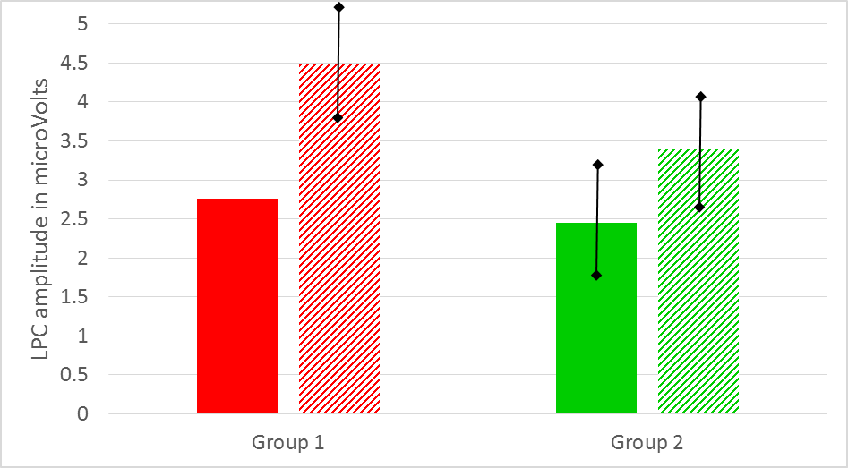
Figure: Mean LPC amplitude in microVolts for group 1 (red) and group 2 (green) as a function of condition (solid vs striped). Note that there is a correspondence with the LPC amplitudes as displayed in Figure 8 (grand average waveforms).