Analysis of Neural oscillations: Step by Step
by Katerina Georgeopoulou en Tonny Mulder

During the recording, your EEG signal can become contaminated by sources other than from the brain, such as the mains grid (our electricity network). This produces a high-amplitude 50 Hz artifact (60 Hz in the USA), often ‘repeated’ at the multiples of the frequency (at 100 Hz, 150 Hz and so on). Furthermore, low frequency drifts can obscure your data.
The first step in the proces is to get rid of these contaminations. There are a few ways to do this. If you are interested in the lower frequencies, say Delta, Theta, Mu, Alpha, Beta or low-Gamma frequencies, you may want to use a band‐pass filter of 0.5 to 48 Hz on your data. In this way, you remove the 50 Hz artifact and a larger part of the slow drifts, while keeping a broader range of frequencies in your data.
Obviously, if you are interested in higher gamma frequencies you should adjust the upper bound of your filter (e.g. use a band‐pass filter of 0.5 to 80 Hz) and apply an additional band‐stop or notch filter to remove the electricity network artifact.
After filtering out the contaminations, your EEG signal typically looks a lot “quieter” and is ready for segmentation into experimental conditions.
Processing TIP
At this early stage it is suggested to keep a broad frequency range into your dataset, eventhough your research question may involve a specific frequency band. For instance, when plotting a time‐frequency graph, it is common to show more than one frequency band. You will fine tune the filtering to the frequency band of your interest in a later stage of the processing.
The next step is to segment the data into your trials.
You have to segment your raw recording into the trials that correspond to your conditions. Most likely you inserted markers to mark onsets of interesting sections. You also have to decide what you will be using as a baseline. It will most likely be in the form of a separate control condition.
Several decisions have to be made, which explains best with an example.
Lets say you are interested in the effect of music on the alpha power of your brain and you have recorded 10 minutes of data (see Figure on the right) with alternating music experimental trials (E1-E5) and silent control trials (C1-C5) of 1 minute each. The most straightforward way to segment this recording is into 10 separate trials. For each individual Control and Experimental trial you calculate the alpha power using the Time-Frequency Tool (See below) and you can compare the average power of the silent trials with the average power of the music trials. So far so good!
The standard power calculation procedure
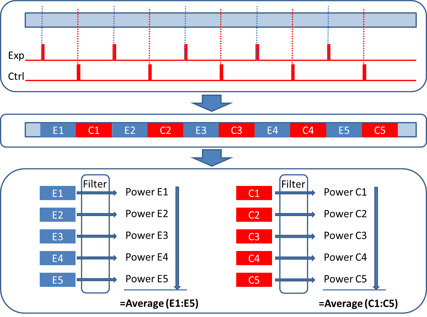
Figure: Segmenting the raw recording into individual trials. On the basis of your triggers (in red) select designated sections from your data and analyse them.
If one or more of your experimental trials is contaminated with artifacts like muscle activity, eye blinks or other movement artifacts, the power calculation of these trials will be compromised and you loose one or several full trials. Elegant ways for artifact detection and removal exist, such as using external electrodes at the eye or muscle areas and applying algorithms to automatically remove the contaminated sections from your data, but our analysis tools do not provide these options. Also you might want to think twice about leaving such a delicate and important proces to 'a machine'.
In case of many short trials, use ERP artifact tool. Identify the 'bad' trials and remove them using Array Manipulator.
In case of a few long trials, removing a full trial is not an ideal solution, because a large amount of data will be lost. Identify the time periods within the trails where the artifacts reside. Use the Time-Frequency tool to manually deselect these periods when constructing average power calculations.
*dit heeft als nadeel dat wanneer je een gemiddelde TF maakt het artefact er wel in wordt meegenomen. Bij genoeg trials/ppn is dat geen probleem. Anders toch overwegen trials te verwijderen.
Another way of removing short sections from a long trial
You may want to consider to segment each trail further into shorter subtrials (see Figure on the right, continuing with the music experiment example). View each of the sub-trials separately (ERP-Artifact Tool) and delete the sub-trial with the eye blinks (Array manipulator). Then calculate the powers of the remaining sub-trials (Time-Frequency tool) and average them for a reliable measurement of the power for the entire trial, saving the day!.
Segmentation into subtrials has a further benefit if you consider that the power of any frequency can ramp up or down within one trial on the basis of what is presented during that period. Think about the JAWS movie!
When artifacts exist
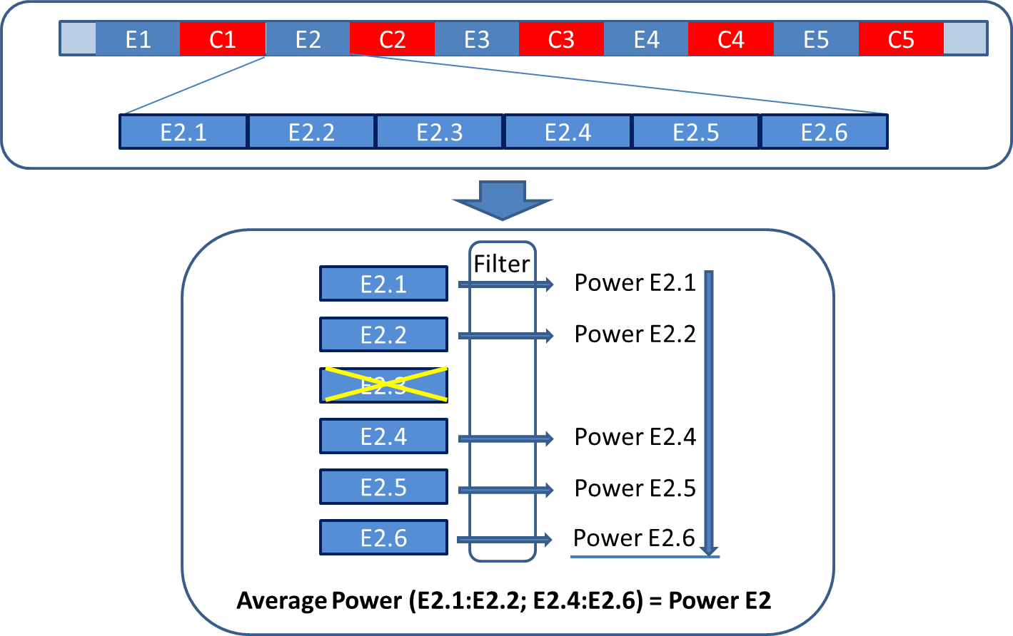
Figure: Deleting sections with artifacts from individual trials without losing your trail.
What if the artifacts are continuously present
In certain cases there are several continuous artifacts of short duration within one trial, such as continuous eye‐blinks. For this course, the suggestion is to carefully inspect your data and reject a trial only when the artifacts exceed a visually acceptable level.
You can ask for assistance if you find this difficult to determine in the beginning. The percentage of total rejected trials per subject should not be too large: 5‐10% is reasonable, but when the rejected trials exceed the 15%, you may consider leaving the participant out of your analysis. Of course, the best method to keep this percentage low is to prevent artifacts by asking your participants to relax their muscles (especially face, neck, arm and shoulder muscles) and not to move or blink if possible.
a. Zorg voor een schone baseline
b. Idealiter baseline periode per trial
c. Wanneer de baseline en time-of-interest (toi) uit elkaar liggen zijn er 2 opties:
i. Baseline en toi apart knippen bij segmentatie stap, en later in de Array Manipulator achter elkaar zetten (in de tijds dimensie). Het gecombineerde bestand kan worden gebruikt voor trial rejection. *Nadelen: hierdoor ontstaan mogelijk ‘edge-artefacts’ waardoor het nodig is om de periode waar ze aan elkaar zijn geplakt niet mee te nemen in de analyse. Dit betekent of een korte baseline en toi, of baseline en trial extra ruim knippen.
ii. Tussenliggende data meenemen in segmentatie stap bij het meten van de power waardes alleen de toi invoeren. *Nadelen: figuur wordt mogelijk minder mooi (bij erg lange trials), tussenliggende artefacten kunnen power-schaal (kleuren) vertekenen, computationeel misschien te zwaar.
THE OLD WAY OF POWER CALCULATION
Now you can calculate the power/energy value of your trials for every channel and frequency band of interest.
Consider the limitations of the Filter tool
The Filter tool handles only 2D data files. So if you have segmented your data into trials, your file might include, Time vs channels vs trials: 3D data files. Load your files into the array manipulator tool to confirm.
To return to 2D data files you might consider to separate each dataset into data sets for each individual channel. So for each channel you have a time vs trails file. Use the array manipulator tool to do this. There are several options.
Please note that you have to keep track of what is in your file, so careful naming is essential
Processing TIP
In the first processing step you have used the FILTER TOOL for a limited number of trials, predominantly in the 'First 8' modus. The tool, however can filter up to 80 trials simultaneously. This means that can use the 'array manipulator tool' to concatinate a number of trials, analysis can speed up. Again, keep track of what you stack into one file.
Averaging
Tool to use: Time-frequency tool. Dit is een nieuwe tool die recent is toegevoegd aan EEG_recorder. gebruik de tool tips en help functie in EEG_recorder zelf. Vraag hulp aan je begeleider
TF per trial berekenen en middelen over trials (TF-tool)
Gemiddeldes per proefpersoon en conditie gebruiken om gemiddelde power te berekenen binnen time-of-interest en frequency-of-interest. (TF-tool)
Grand average maken: gemiddeldes per persoon opslaan in TF-tool en samenvoegen in Array-Manipulator. Dit gecombineerde bestand inladen in TF-tool en middelen over proefpersonen.
The old way of doing it
Calculate the power with the filtertool and average powers with excel
Then, you can average the trials per participant and per condition. Example: suppose you have 9 participants and 3 conditions, with 5 trials in each condition. You then average the 5 trials per condition together, so that you end up with 9 x 3 values (one average value for every participant and condition). If you are looking at several channels and/or frequency bands, you repeat this step separately for each. Finally, you can test if the values differ statistically between the conditions, and you can do this separately for every frequency band and channel.
Presenting the results.
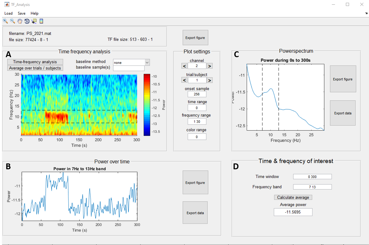
Tool to use in recorder: TF-Tool
Tool modal to be created
Next to the statistical results, you can also look at time‐frequency plots of your data. These are colored graphs with time on the x‐axis and the frequencies on the y‐axis. The color indicates the power/energy of a frequency at a specific time point (e.g. red for higher values for power/energy and blue for lower values). The advantage of time‐frequency plots is that they contain both time and frequency information. In other words, they can show how frequencies change during the time course of your experiment, while a mean value of power/energy is much more static. An example: suppose that in condition 1, your subjects show more alpha power/energy in the beginning of the trial and less alpha power/energy in the end, while the opposite is true for condition 2. The average value for alpha power/energy may then be the same for both conditions, leading you to think that there is no difference between the conditions. However, the time‐frequency plot will reveal that two different processes may be taking place. Another advantage of the time‐frequency plot is that it helps you detect interesting phenomena in other frequency bands or dynamics between frequencies. For instance, you may notice that beta power/energy gradually increases whenever alpha power/energy diminishes and this may lead you to further conclusions. For these reasons, the timefrequency plot is a useful visual tool and a valuable addition to your presentation or paper.